What is polynomial regression

Our friend Timmy gave us some data composed of input into a system and the corresponding output from the system. We will refer to the input as the independent variable (x) and the output as the dependent variable (y). We plot the data on an x versus y scatter plot.

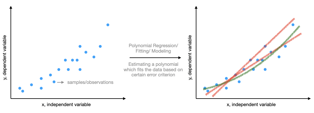
The plot on the left looks neat. We know some high school mathematics and so start to wonder can we fit a polynomial to this data. That is, can we write y as follows:

$$y = \sum_{p=1}^{P}a_{p}x^{p}+w$$

where P is the order of the polynomial, a_p are the polynomial coefficients, and w is what could not be modeled by the polynomial (or noise). Examples of these fits are shown in the right plot. But why do we fit anything to the data given by Timmy? The simple answer is - we are curious and we know little math, and there are good tools at are service to do this. Remember, F. Gauss, the famous, also did this when he collected astronomy data, and his tools were much more laborious (pen and paper). Coming back, this curiosity may lead us to identify some relationship between input and output. What happens when you discover a relationship? The output does not looks random anymore, and given an input you can predict something close to what the system will output. Depending on the data you are trying to model (or Timmy gave), this can be amazing. It can help you understand the system or predict outputs and devise actions.

How is it done

Lets ask - How can when say the polynomial is a bad fit? In short, we have to first quantify what is good or bad here. Given an input x, we obtain the difference between the true output and polynomial model output. This is the error. The sign of the error is not a concern so we square this error. The squaring also make the error (as a function of input, a_p) a differentiable function. We sum this error over all N samples. That is,

$$E = \sum_{n=1}^{N}(y[n]-y_{hat} [n])^2$$ $$y_{hat}[n]= \sum_{p=1}^{P}a_{p}x^{p}[n]$$

We will say the fit is good if the error is low. Again, low is qualitative, lower the better. But how much low is okay? Well, this depends on the application.

How will we do it here - Gradient Descent

We will use high school calculus, specifically, derivative. The derivative of a curve at any point gives the slope at that point. This is useful in many ways and particularly for our error function E, introduced above. The error function E is quadratic in a_p, and that means it is convex and reaches a minimum at a specific point in the multi-dimensional plane defined by a_ps. That's a good thing. We can start at any random point in this space, and compute derivative, and slide along the direction where the E decreases. This algorithm is referred to as gradient descent. Do read more about it - it is simple and quite powerful for wide varieties of problems.

We will use pytorch to implement this regresison using gradient descent. Lets start. I learnt this while listening to a course in fast.ai.

import numpy as np
import torch
import matplotlib.pyplot as plt
from matplotlib.ticker import (MultipleLocator, FormatStrFormatter,
                               AutoMinorLocator)
import torch.nn as nn
import torch.tensor as tensor

Create the dataset as a sum of a third degree polynomial and a little bit of uniform random noise.

# make the data
n = 100 # number of samples of x
x = torch.ones(n,4) # make a tensor
x[:,0].uniform_(-1,1) # x 
x[:,1] = x[:,0]**2
x[:,2] = x[:,0]**3
a = tensor([1.,1,1,5]) # polynomial coefficients
amax = 1
amin = -1
# create dataset y
y = x@a + (amax-amin)*torch.rand(n)+amin # sum of polynomial and uniform random noise [-1,1]

So, Timmy has given us y and x. Let's visualize it on a scatter plot. We will also overlay on the scatter plot the samples from the underlying polynomial model governing this system. Ideally, we will like our polynomial regression to exactly match this polynomial model. If this happens then we have understood the system exactly.

fig = plt.subplots(figsize=(6,4))
ax = plt.subplot(1,1,1)

ax.scatter(x[:,0],y,label='experiment samples')
ax.scatter(x[:,0],x@a,label='underlying polynomial model samples')
ax.grid(True)
ax.spines['right'].set_visible(False)
ax.spines['top'].set_visible(False)  
ax.tick_params(which='both', width=2)
ax.tick_params(which='major', length=7)
# ax.tick_params(which='minor', length=4, color='gray')
ax.legend(loc='upper left',frameon=False,fontsize=14)
plt.xticks(fontsize=13)
plt.yticks(fontsize=13)
ax.set_xlabel('x',fontsize=14)
ax.set_ylabel('y (x)',fontsize=14)
plt.tight_layout()

Implementation

# Lets implement the error function
def mse(y_hat,y):
    return((y_hat-y)**2).mean()

# Lets initialize our polynomial model
a_hat = torch.tensor([1.,1.,0,0])
a_hat = nn.Parameter(a_hat)

# Lets define our gradient descent updates
accumulate_loss = []
def update():
    y_hat = x@a_hat # estimate y_hat
    loss = mse(y,y_hat) # compute error or loss
    accumulate_loss.append(loss)
#     if t % 10 == 0: print(loss)
    loss.backward() # compute derivative/grad with respect to each parameter
    with torch.no_grad(): # deactivate backprop
        a_hat.sub_(lr*a_hat.grad) # gradient descent step
        a_hat.grad.zero_() # reset grads
lr = 1e-2 # this is learning rate parameter, if curious, do google more on it 
for t in range(1000): update()

Lets visualize the loss curve over updates, and the estimated model overlaid on the true model.

fig = plt.subplots(figsize=(14,4))
ax = plt.subplot(1,2,1)
ax.plot(np.array(accumulate_loss)*1e6)
ax.grid(True)
ax.spines['right'].set_visible(False)
ax.spines['top'].set_visible(False)  
ax.tick_params(which='both', width=2)
ax.tick_params(which='major', length=7)
plt.xticks(fontsize=13)
plt.yticks(fontsize=13)
ax.set_xlabel('update index',fontsize=14)
ax.set_ylabel('Loss x 1e6',fontsize=14)
plt.tight_layout()

ax = plt.subplot(1,2,2)
ax.scatter(x[:,0],y,label='experiment samples')
ax.scatter(x[:,0],x@a,label='underlying polynomial model samples')
ax.scatter(x[:,0],x@a_hat.detach().numpy(),color='g',label='estimated polynomial model samples')

ax.grid(True)
ax.spines['right'].set_visible(False)
ax.spines['top'].set_visible(False)  
ax.tick_params(which='both', width=2)
ax.tick_params(which='major', length=7)
# ax.tick_params(which='minor', length=4, color='gray')
ax.legend(loc='upper left',frameon=False,fontsize=14)
plt.xticks(fontsize=13)
plt.yticks(fontsize=13)
ax.set_xlabel('x',fontsize=14)
ax.set_ylabel('y (x)',fontsize=14)
plt.tight_layout()

From the above plots it is clear that we are headed in the descent direction (decresing loss or error). Further, our estimated polynomial model closely follows the underlying true polynomial model.

print('True model coefficients:')
print(a.numpy())
print('Estimated model coefficients:')
print(a_hat.detach().numpy())

True model coefficients:
[1. 1. 1. 5.]
Estimated model coefficients:
[1.1652924 0.9945537 0.5666001 5.0914917]

That's it

We saw that gradient descent can be used to estimate the coefficients of a linear regression model. Traditionally, polynomial regression is done using the Moore Penrose inverse. But we tried here using a NN approach and it too works and approximates the traditional solution. The flexibility here is we can use different differentiable error functions are obtain variants of the regression.