A short tale on the longest day
Are some days really short and some long?


About
I had forgotten about the longest day. But now since 2017, around 21st June, I always notice in social media some news about it. Now, to further strengthen my excitement, I have my nephew who shares the birthday with summer solstice, and also two wonderful friends whose birthdays are one day before and one day after this day.
This time I read an exciting story shared by Vishu Guttal here. He describes his visit to a school and an exercise he did school students on verifying the "longest day" fact. I was amazed on reading it, and suggest you too! Subsequently, I thought of doing the exercise myself. This post is a result of that.
Astronomy is amazing. You can make theory, prediction, observations, and verification - but all this without ever getting close to the entity you are studying. This science has amazed humanity for centuries - Does earth go around the Sun? Is the orbit elliptical? Are there many galaxies? Is the universe expanding? Did all this start with a big bang? - Theories have been made, verified, approved, disapproved, and updated. That’s the definition of science.
Let's take a very small ride into this field as we sit (or stand, whatever you are doing) and verify - the "longest day" fact by crunching some numbers and plotting the data.
First let's list a few other known facts.
- Earth goes around Sun
- This path is elliptic
- Earth is tilted about its axis
It is not easy to verify these three bullets. Spare a moment, and imagine staring at the sky, and verifying the above statements. It is not easy, and you will thank some amazing folks who did this. As a result of these facts we now understand why we experience on Earth:
- seasons
- a longest day and a shortest day
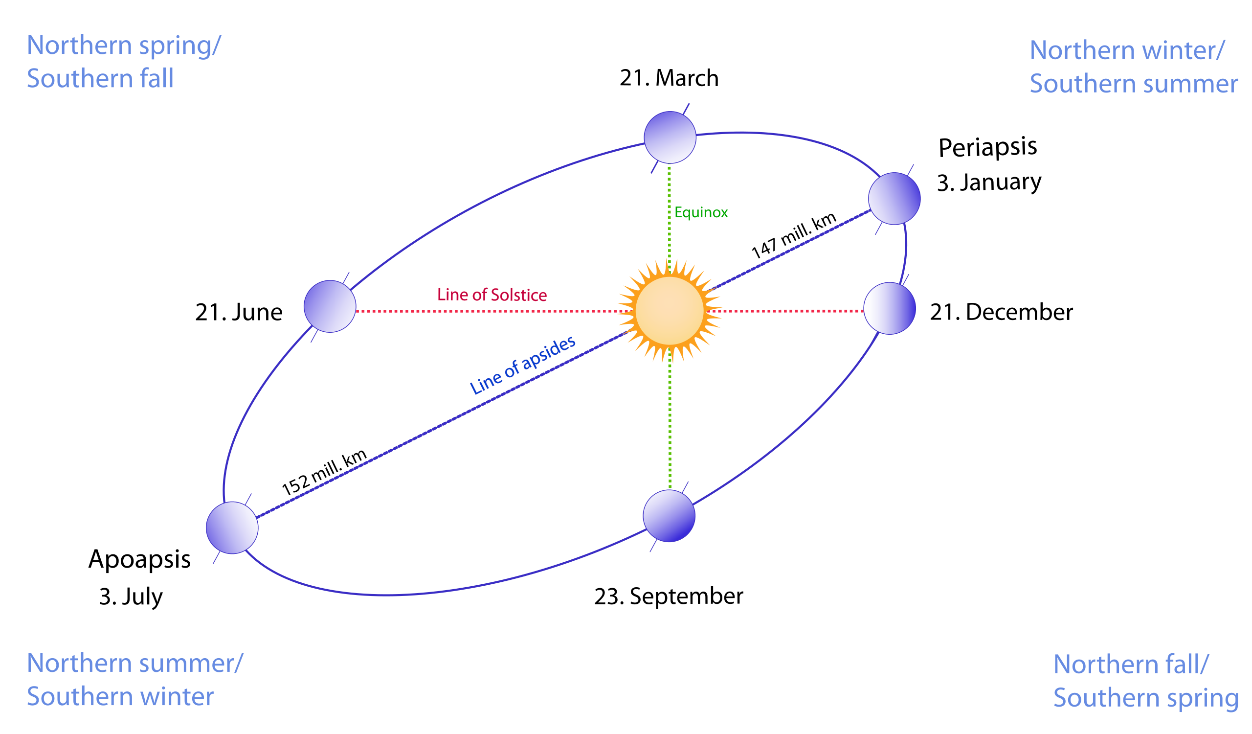
Intuitively, the season should be determined by length of the day. A longer day will imply more heat incident on the Earth surface, indicating a day in summer. The below figure from Wikipedia helps understanding this. The interesting thing to note is that summer is not when earth is closest to the Sun. This is because of the tilt of the Earth. Owing to this tilt we have a day of the year on which the northern hemisphere is exposed to the Sun for maximum time, while the Earth rotates around its own axis. This day is called the summer solstice. Similarly, we have a day of winter solstice - shortest day.
So why did the Earth tilt? One theory states - Long long time ago something came flying by and hit Earth, and since then, our Earth got tilted! To read more click here. The nice thing is thus, we have seasons!
Can you think of how we can verify the longest day claim. Spare a few moments. In the code below we will do a small exercise to verify that there exists a longest day. We will do this for just one year, 2019. The same thing can be done for any year if you are in doubt. The idea is simple.
- Using python we will write few lines of codes
- This will use "astral package" to find the sunrise/sunset times for any latitude (and longitude) on Earth.
- We will visualize this data
Fingers crossed on what the plots will look like, let's keep scrolling.
#collapse
# import some packages
import pandas as pd
import numpy as np
import datetime
import matplotlib.pyplot as plt
import time
from astral import LocationInfo
from astral import sun
import pytz
from mpl_toolkits.axes_grid1 import make_axes_locatable # to move placement of colorbar
from matplotlib.ticker import (MultipleLocator, FormatStrFormatter,
                               AutoMinorLocator)
Step 1: We will load a CSV file which contains the latitude and longitude location of 212 cities in India. This is good as we can visualize the sunrise/sunset times across India, particularly, from East to West.
#collapse
# load indian cities dataset
df = pd.read_csv('./my_data/indian_cities_lat_long.csv')

# sort rows from east to west (that is, longitude values)
df = df.sort_values('lng',ascending=False)
df = df.reset_index(drop=True)
Step 2: We will make a variable containing all dates of 2019
#collapse
# get all dates in 2019
start = datetime.datetime(2019, 1, 1, 0, 0, 0)
end = datetime.datetime(2019, 12, 31, 0, 0, 0)
delta = end - start
Step 3: We will call the astral package and compute the sunset/sunrise time for all 212 cities for all 365 days of 2019.
#collapse
data = {}
data['sunrise'] = []
data['sunset'] = []
data['noon'] = []

for cnt in range(len(df)):
    data['sunrise'].append([])
    data['sunset'].append([])
    data['noon'].append([])
    i = 0
    for day in range(delta.days + 1):
        t_start = time.time()
        this_date = str((start+datetime.timedelta(days=day)).date())
        params = {'lat':df['lat'][cnt],'lng':df['lng'][cnt],'date':this_date}
        tz = pytz.timezone('Asia/Kolkata')
        l = LocationInfo()
        l.name = 'name'
        l.region = 'region'
        l.latitude = df['lat'][cnt]
        l.longitude = df['lng'][cnt]
        s = sun.sun(l.observer, date=start+datetime.timedelta(days=day),tzinfo=tz)
        data['sunrise'][cnt].append(s["sunrise"].time().strftime('%H:%M:%S'))
        data['sunset'][cnt].append(s["sunset"].time().strftime('%H:%M:%S'))
        data['noon'][cnt].append(s["noon"].time().strftime('%H:%M:%S'))
Step 4: Some data structuring into numpy arrays to ease later visualization.
#collapse
sun_rise_in_secs = []
sun_set_in_secs = []
sun_overhead_in_secs = []
sun_length_in_secs = []

for i in range(len(data['sunrise'])):
    sun_rise_in_secs.append([])
    sun_set_in_secs.append([])
    sun_overhead_in_secs.append([])
    sun_length_in_secs.append([])

    for j in range(len(data['sunrise'][0])):
        time_1 = data['sunrise'][i][j].split(':')
        time_2 = data['sunset'][i][j].split(':')
        time_3 = data['noon'][i][j].split(':')

        sun_rise_in_secs[i].append(float(time_1[0])*60*60+float(time_1[1])*60+float(time_1[2]))
        sun_set_in_secs[i].append(float(time_2[0])*60*60+float(time_2[1])*60+float(time_2[2]))
        sun_overhead_in_secs[i].append(float(time_3[0])*60*60+float(time_3[1])*60+float(time_3[2]))
        sun_length_in_secs[i].append(sun_set_in_secs[i][j]-sun_rise_in_secs[i][j])

sun_rise_in_secs  = np.array(sun_rise_in_secs)
sun_set_in_secs  = np.array(sun_set_in_secs)
sun_overhead_in_secs  = np.array(sun_overhead_in_secs)
sun_length_in_secs  = np.array(sun_length_in_secs)

# np.argmax(daylength_in_secs,axis=1)
#collapse
# plot daylength
day_max = np.argmax(sun_length_in_secs,axis=1)+1
# date_max = []
# for i in range(len(day_max)):
#     date_max.append(datetime.datetime(2019, 1, 1) + datetime.timedelta(day_max[i] - 1))

fig = plt.subplots(figsize=(16,7))
ax = []
ax.append(plt.subplot(1,1,1))
ax[0].plot([14,14],[9,15],'--',color='blue',linewidth=2,alpha=0.8)
ax[0].plot([171,171],[9,15],'--',color='blue',linewidth=2,alpha=0.8)
ax[0].plot([355,355],[9,15],'--',color='blue',linewidth=2,alpha=0.8)
ax[0].plot([0,365],[12,12],'--',color='green',linewidth=2,alpha=.8)
# ax[0].plot(sun_length_in_secs.T/60/60,alpha=0.4)
ax[0].plot(sun_length_in_secs[0]/60/60,color='tab:red',linewidth=5,label=df['city'][0])
ax[0].plot(sun_length_in_secs[-1]/60/60,color='tab:blue',linewidth=5,label=df['city'][len(df)-1])
ax[0].text(2,13,'15th Jan',rotation=90,fontsize=14)
ax[0].text(158,13,'21st June',rotation=90,fontsize=14)
ax[0].text(342,13,'21st Dec',rotation=90,fontsize=14)
ax[0].set_xlabel("DAYS SINCE 1st JAN",fontsize=14)
ax[0].set_ylabel("DAYLIGHT DURATION [in hrs]",fontsize=14)
ax[0].grid(True)
ax[0].spines['right'].set_visible(False)
ax[0].spines['top'].set_visible(False)
ax[0].xaxis.set_minor_locator(AutoMinorLocator())
ax[0].yaxis.set_minor_locator(AutoMinorLocator())
ax[0].tick_params(which='both', width=2)
ax[0].tick_params(which='major', length=7)
ax[0].tick_params(which='minor', length=4, color='gray')
ax[0].legend(frameon=False, fontsize=14)

# im = ax[1].imshow(sun_length_in_secs/60/60, cmap='RdBu_r')
# ax[1].set_xlabel("DAYS SINCE 1st JAN",fontsize=14)
# ax[1].set_ylabel("CITIES",fontsize=14)
# divider = make_axes_locatable(ax[1])
# colorbar_ax = fig.add_axes([.92, 0.2, 0.01, 0.5])
# cbar = fig.colorbar(im, cax=colorbar_ax)
# cbar.set_label('DAY LENGTH [in hrs]',size=13)
# ax[1].plot(day_max-1,np.arange(0,sun_length_in_secs.shape[0],1),'o-',color='k')
# yticks = [0,50,100,150,200]
# keys = []
# for i in range(len(yticks)):
#     keys.append(df['city'][yticks[i]])
# ax[1].set_yticks(yticks)
# ax[1].set_yticklabels(keys,rotation=0,fontsize=13)
plt.show()
You can see that there is a nice peak around 21st June for the day length data. This peak is there in traces for all the 212 cities, and the patterns is similar. For the majority of the cities this happens to be exactly 21st June. Here, Dibrugarh is the eastern most city in our database, and Porbandar is the westernmost. The interesting thing is also the variation in the trace of day length across the cities. Also, note that there are two days of the year on which day length is exactly 12 hrs! These dates correspond to the equinox.
Next, let's visualize the sunrise times for all 365 days. The code is given below.
#collapse
fig, ax = plt.subplots(1,2,figsize=(16,7))
ax[0].plot(sun_rise_in_secs.T/60/60,alpha=0.4)
ax[0].plot(sun_rise_in_secs[0]/60/60,color='k',linewidth=5,label=df['city'][0])
ax[0].plot(sun_rise_in_secs[-1]/60/60,color='r',linewidth=5,label=df['city'][len(df)-1])
ax[0].set_xlabel("DAYS SINCE 1st JAN",fontsize=14)
ax[0].set_ylabel("SUNRISE [in hrs]",fontsize=14)
ax[0].grid(True)
ax[0].spines['right'].set_visible(False)
ax[0].spines['top'].set_visible(False)
ax[0].xaxis.set_minor_locator(AutoMinorLocator())
ax[0].yaxis.set_minor_locator(AutoMinorLocator())
ax[0].tick_params(which='both', width=2)
ax[0].tick_params(which='major', length=7)
ax[0].tick_params(which='minor', length=4, color='gray')
ax[0].legend()

im = ax[1].imshow(sun_rise_in_secs/60/60, cmap='RdBu_r')
ax[1].set_xlabel("DAYS SINCE 1st JAN",fontsize=14)
ax[1].set_ylabel("CITIES",fontsize=14)
divider = make_axes_locatable(ax[1])
colorbar_ax = fig.add_axes([.92, 0.2, 0.01, 0.5])
cbar = fig.colorbar(im, cax=colorbar_ax)
cbar.set_label('SUNRISE [in hrs]',size=13)
yticks = [0,50,100,150,200]
keys = []
for i in range(len(yticks)):
    keys.append(df['city'][yticks[i]])
ax[1].set_yticks(yticks)
ax[1].set_yticklabels(keys,rotation=0,fontsize=13)
plt.show()
#collapse
fig, ax = plt.subplots(1,2,figsize=(16,7))
ax[0].plot(sun_set_in_secs.T/60/60,alpha=0.4)
ax[0].plot(sun_set_in_secs[0]/60/60,color='k',linewidth=5,label=df['city'][0])
ax[0].plot(sun_set_in_secs[-1]/60/60,color='r',linewidth=5,label=df['city'][len(df)-1])
ax[0].set_xlabel("DAYS SINCE 1st JAN",fontsize=14)
ax[0].set_ylabel("SUNSET TIME [in hrs]",fontsize=14)
ax[0].grid(True)
ax[0].spines['right'].set_visible(False)
ax[0].spines['top'].set_visible(False)
ax[0].xaxis.set_minor_locator(AutoMinorLocator())
ax[0].yaxis.set_minor_locator(AutoMinorLocator())
ax[0].tick_params(which='both', width=2)
ax[0].tick_params(which='major', length=7)
ax[0].tick_params(which='minor', length=4, color='gray')
ax[0].legend()

im = ax[1].imshow(sun_set_in_secs/60/60, cmap='RdBu_r')
ax[1].set_xlabel("DAYS SINCE 1st JAN",fontsize=14)
ax[1].set_ylabel("CITIES",fontsize=14)
divider = make_axes_locatable(ax[1])
colorbar_ax = fig.add_axes([.92, 0.2, 0.01, 0.5])
cbar = fig.colorbar(im, cax=colorbar_ax)
cbar.set_label('SUNSET [in hrs]',size=13)
yticks = [0,50,100,150,200]
keys = []
for i in range(len(yticks)):
    keys.append(df['city'][yticks[i]])
ax[1].set_yticks(yticks)
ax[1].set_yticklabels(keys,rotation=0,fontsize=13)
plt.show()
#collapse
fig, ax = plt.subplots(1,2,figsize=(16,7))
ax[0].plot(sun_overhead_in_secs.T/60/60,alpha=0.4)
ax[0].plot(sun_overhead_in_secs[0]/60/60,color='k',linewidth=5,label=df['city'][0])
ax[0].plot(sun_overhead_in_secs[-1]/60/60,color='r',linewidth=5,label=df['city'][len(df)-1])
ax[0].set_xlabel("DAYS SINCE 1st JAN",fontsize=14)
ax[0].set_ylabel("NOON [in hrs]",fontsize=14)
ax[0].grid(True)
ax[0].spines['right'].set_visible(False)
ax[0].spines['top'].set_visible(False)
ax[0].xaxis.set_minor_locator(AutoMinorLocator())
ax[0].yaxis.set_minor_locator(AutoMinorLocator())
ax[0].tick_params(which='both', width=2)
ax[0].tick_params(which='major', length=7)
ax[0].tick_params(which='minor', length=4, color='gray')
ax[0].legend()

im = ax[1].imshow(sun_overhead_in_secs/60/60, cmap='RdBu_r')
ax[1].set_xlabel("DAYS SINCE 1st JAN",fontsize=14)
ax[1].set_ylabel("CITIES",fontsize=14)
divider = make_axes_locatable(ax[1])
colorbar_ax = fig.add_axes([.92, 0.2, 0.01, 0.5])
cbar = fig.colorbar(im, cax=colorbar_ax)
cbar.set_label('NOON [in hrs]',size=13)
yticks = [0,50,100,150,200]
keys = []
for i in range(len(yticks)):
    keys.append(df['city'][yticks[i]])
ax[1].set_yticks(yticks)
ax[1].set_yticklabels(keys,rotation=0,fontsize=13)
plt.show()
Here we see something which I didn't expect. India has one timezone and hence, we see a gradual increase in noon time from east to west. But what are those sinusoidal patterns, and also there is a downward moving trend.
That's it
We verified that there does exist a longest day around 21st June. For the majority of the cities this day was 21st June, and for a few others it was 20 or 22 June. Also, we did not verify here, but it appears that around 21st June the day lengths differ by a few seconds.
Twice in a year the day length is equal to the night length.
The noon time varies across the year in a pattern which does seem interesting.
On top of this, I also find it interesting that we can estimate the sunrise/sunset/noon times using some math equations. There is a wiki article on this. I will try to know more about this sometime. As of now, I would like to thank the astral package for the implementation. I tried first using a free API but the query to get the data was taking time in hrs. I will also like to than Vishu Guttal for sharing the nice initiative and also publishing it in Resonance, a Science Communication journal.